Did Your Model See This Coming?: The Science Behind a Question We're Always Asked

What You Should Know

Verification and validation of high-resolution, downscaled climate model data are an essential part of providing decision-grade climate risk analytics. But the process is widely misunderstood — and those misunderstandings have real consequences for how climate data gets evaluated, trusted, and used.

Jupiter's verification and validation process takes a different approach: dozens of individual checks, both automated and reviewed by leading scientific experts, run against 251 trillion data values. That transparent, comprehensive, quantifiable, and well-documented process has enabled ClimateScore Global™ to pass Model Risk Management (MRM) validation at Tier 1 banks — allowing for the rapid adoption of decision-ready climate risk analytics.

This series will explore the verification and validation process in detail for several specific perils: fire, flood, and wind.

Verifying and Validating Climate Models

What Is a Climate Model?

Climate model data is the backbone of climate risk analytics. But what is a climate model, really? At their heart, global climate models (GCMs) use computers to solve the mathematical equations that describe the physical processes that govern Earth’s climate system. Think: equations such as the first law of thermodynamics, or the Navier-Stokes equations that describe how fluids (such as the atmosphere and the ocean) move. Overall, GCMs contain millions of lines of code solving hundreds of equations to model various aspects of the Earth’s climate system, including the atmosphere, ocean, glaciers and sea ice, and land surface.    

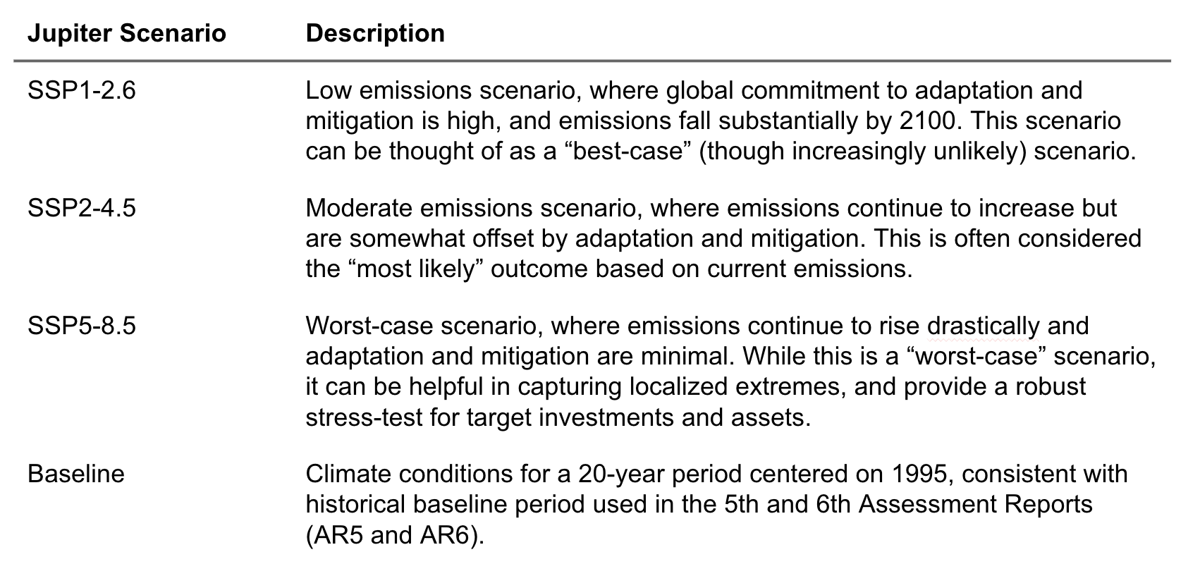
Global climate models are used to simulate Earth’s climate system, both historically and in the future. They are primarily used to model and understand the many ways in which Earth’s complex global climate system can evolve in the future as it responds to changing greenhouse gases and other aerosols. These future GCM results are represented by different scenarios. The Intergovernmental Panel on Climate Change’s 6th Assessment Report (IPCC AR6¹) uses several different scenarios, which GCMs simulate. Jupiter uses 3 of these scenarios (see Table 1), plus an historical baseline scenario. By using the same scenarios with different GCMs, we can understand how GCM outputs might differ in response to standard inputs. 

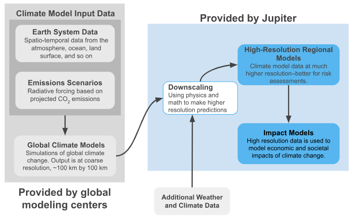
The global climate models are used in key global climate assessments, such as the IPCC AR6. Computational and data storage constraints mean that GCMs are typically run at about 1° latitude by 1° longitude, a resolution that’s too coarse for many decision makers and stakeholders. Thus, many decision makers elect to use higher-resolution models tailored for their region or area of interest. Climate data providers like Jupiter use the process of downscaling to create higher-resolution simulations from GCMs. Bias correction and downscaling models use a variety of physical, statistical, and artificial intelligence methods as well as additional weather and climate data to make high-resolution, calibrated climate predictions. These high-resolution model results are ultimately used to model the economic and societal impacts of extreme weather and climate hazards. 

Throughout the process of creating these high-resolution downscaled climate models, there are several sources of uncertainty in their predictions. There is uncertainty from the GCM data itself, and additional uncertainty introduced in the downscaling process. 

Climate Model Uncertainty: Why We Need Verification and Validation

A full understanding of climate model predictions includes understanding uncertainty around these predictions. For GCMs, uncertainty is typically broken down into three components ^2,3: 

• Natural variability. The Earth’s climate has some level of natural variability that is not directly impacted by human activity. Some summers are very hot and dry, others are cooler and wetter. In some years, there are so many hurricanes that the National Hurricane Center has to use Greek letters; other years see far fewer hurricanes. Well-calibrated GCMs and high-resolution climate models are generally able to capture this natural variability. 
• Scenario uncertainty. Scenario uncertainty is the uncertainty associated with human activities and their greenhouse gas emissions. Scenario uncertainty is addressed by analyzing the GCM results from several different emissions scenarios (see Table 1 for a list of scenarios used in Jupiter climate risk products). 
• Global climate model uncertainty. GCMs solve complex equations with different numerical approximations; GCMs also must approximate physical processes that are very small, or occur very quickly (e.g., the formation of small cumulus clouds). GCMs also choose to approximate these processes in different ways. After all of these approximations, climate scientists must ensure that the GCM output is a faithful representation of the climate system. 

Uncertainty from downscaling. The additional physical, mathematical or AI simulations used in downscaling can introduce further uncertainty. While the downscaling process itself is typically not the major source of uncertainty in downscaled climate model projections ⁴, it can be important in certain situations, such as in areas with complex terrain.   

Robust Evaluation of Climate Risk Data Requires Verification and Validation

Assessing the quality of future predictions is challenging. For weather forecast models, new ground truths are available every day, or even every few hours, giving model developers many opportunities to evaluate their predictions and adjust and improve models accordingly. But how do you evaluate climate model predictions for 2050 in 2026? The key lies in the verification and validation pipeline.

Verification and validation are distinct processes, both essential for ensuring that climate risk data is trustworthy and decision-grade. Verification consists of making sure a model is internally consistent, that it is applying physics correctly, that the model’s code is running properly, and so on. Validation is the process of assessing how well a model represents the real world by comparing it to independent observations.    

Quantifying the quality and reliability of underlying climate model data is critical for climate risk analysis. At Jupiter, verification and validation is an evolving, transparent, and rigorous process by which we test all data we produce. And while quantitative verification and validation is an essential part of the process, so too is human oversight. Jupiter scientists inspect the verification and validation pipeline at every step, designing the pipelines and ensuring that results are reasonable, accurate, and in harmony with the state of the science. With transparent and comprehensive validation and verification, end users can feel confident that the insights within their climate analytics are providing the accuracy and reliability necessary for decisionmaking. 

Common Misconceptions About Verification and Validation

There is no single “right” way to undertake verification and validation for something as complex as the climate model data used for climate risk modeling. The verification and validation processes require a mix of quantitative analysis and expert judgement, and can depend on the ultimate applications and goals of the climate risk analysis. However, there are several commonly held misconceptions about verification and validation, which we will discuss here. We note that the phrase “climate models” refers to the high-resolution, downscaled climate model data produced by Jupiter and other climate data providers. We will use the abbreviation “GCMs” to refer to the coarser, global climate models used to produce the IPCC AR6. 

Climate models are not the same as weather models. Weather forecast models make predictions for specific weather events spanning the next couple of hours out to about two weeks. High quality, real-time data from weather observation systems and satellites are essential for weather forecast models. These data allow the computer model to solve the equations that predict how the weather might evolve in the coming hours and days based on the most recent observations. GCMs and climate models, on the other hand, are constructed to simulate the Earth system over decades or longer. These models don’t predict specific events, but rather, the overall state of the climate including its mean and variability. While weather and climate models use similar types of data and solve many of the same physical equations, they address different types of questions. A weather forecast model can tell you “Do I need to cover my plants this afternoon?” or “should I pack an umbrella for my weekend trip?”. A more appropriate question for a climate model would be,  “will my hometown be hotter in 20 years?” or “will swings between hot and cold periods be more abrupt?”

Climate models do not make deterministic forecasts of specific individual historical events. One of the most common questions we are asked is “Did your model predict *insert specific event*?” A weather forecast model can be run with historical observational data to create a simulation of a specific, historic hurricane, such as 2022’s Hurricane Ian. Climate models, by contrast, are not constantly rerun with snapshots of today’s weather. Because they do not know about today’s weather, they cannot predict events coinciding with reality tomorrow, or in two weeks. Instead, the goal of climate models is to simulate the full range of possible events. That is, a well-calibrated climate model could tell you that a hurricane with the intensity and rainfall of Ian was possible in southwest Florida, but not that Hurricane Ian would hit southwest Florida in September 2022.  

The goal of climate model validation should be thought of as sufficiently sampling the full variability of the climate system. In this way, we can feel confident that the climate model is capable of representing a specific event. So instead of asking “Did a climate model predict this specific hurricane?”, reframe the question: “In a well-validated climate model dataset, could you have expected this event to happen at some probability threshold?” 

Climate models should capture every event we’ve observed in the past. Climate modelers must also avoid overfitting; that is, overly fine-tuning climate models to specific events, sets of events, or locations. A good climate model balances accuracy with generalizability, or the ability to still model the climate system reliably even under conditions not seen before. 

Overfitting can take many forms, but one of the most common is to overly adjust GCMs to match the past perfectly. Sometimes, models can be adjusted so that they model historical climate extremely well – but at the expense of being able to skillfully model future climate states. Furthermore, many geophysical processes can take a long time to go through a full cycle. Solar cycles take 11 years, while some forms of ocean variability vary over decades. Is a model that’s only trained on 20 years of data fully sampling all the possible climate states? Probably not.  

Additionally, weather and climate observation data do not cover the entire globe equally. For example, the United States and the European Union have over 600 weather radar stations covering 1.1 billion people, while the 1.2 billion people living in Africa are served by just 37 radars⁵. And many weather observing stations in the Global South have records of fewer than 30 years, meaning the full range of climate variability has likely not been sampled^3,6. This reduced data quality and coverage can lead to certain regions, such as the U.S., Europe, Australia, and Japan, being overrepresented in GCM data, while other regions such as South America, Africa, and Southeast Asia being underrepresented.  

Several forms of overfitting are unique to downscaled climate model data. One is the errors introduced by the statistical and artificial intelligence methods used in downscaling climate model data. These methods, which take lower-resolution data and make it higher-resolution and more localized, can be especially vulnerable to overfitting. The approaches excel at identifying complex patterns in large amounts of data. However, overly complex statistical, and especially AI approaches, can sometimes prioritize memorizing random fluctuations in the data, rather than real physical relationships. Then, when models go to predict rare events, or events far in the future, they have memorized noise instead of physics, and their predictions fail. Good statistical or AI models are constructed with techniques that prioritize simplicity and generalizability and discourage overfitting; however, the best defense is always human expertise.

Downscaled climate model data is also at risk of false precision. Decision-makers often dream of climate risk predictions at the resolution of individual buildings, or even higher resolution. The reality is that the underlying data and methods – GCM data, digital elevation models, and so on – often do not support making predictions at such high resolution. Even though this data can be produced computationally, it is vulnerable to false precision – the misleading sense of high accuracy. This high-resolution data may look good, but it can lead decision-makers astray.       

Multiple model averages are better than a single model. Statisticians are familiar with the saying credited to George Box that “All models are wrong, but some are useful”. This is certainly true in climate modeling. GCMs must account for processes on huge varieties of spatial scales across many Earth systems – from cloud droplet formation that takes place in seconds to slow-varying ocean dynamics. With such a variety of processes, climate model developers are invariably forced to make decisions about computation, software engineering, and parameterizations – mathematical approximations for processes that are too small, fast, or nonlinear to be simulated directly. 

Furthermore, different GCMs are developed by different modeling groups. These groups of experts can make different, but valid, choices in terms of datasets, mathematical approximations, and other model development choices. These choices ultimately result in a range of climate outcomes, giving climate data providers a broad set of possibilities to study. Possibly counter-intuitively, the complexity of the climate modeling process is sufficiently complex that many models share common elements, and even code. This means some models naturally group because their strengths and weaknesses are similar.

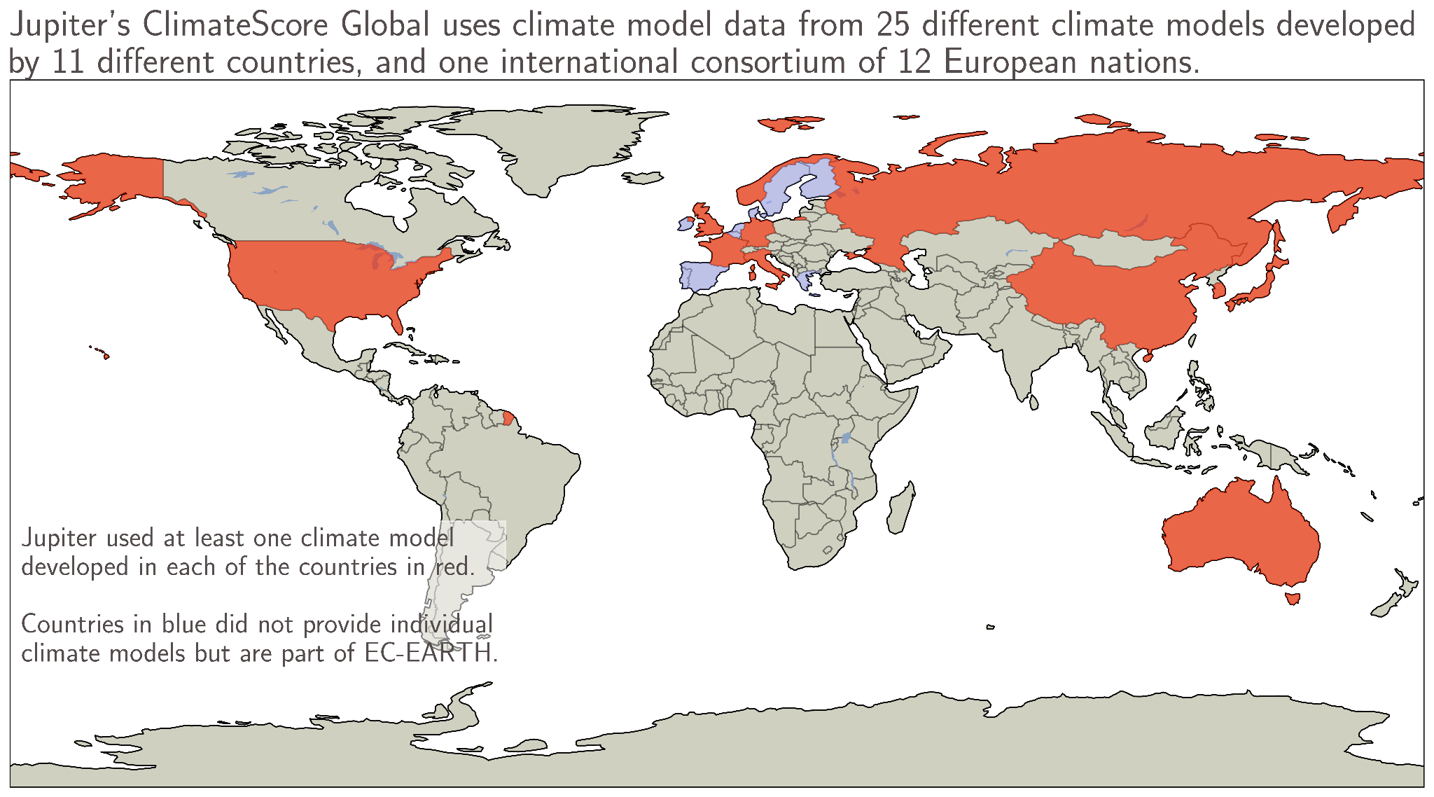
At Jupiter, model simulations from both the 5th and 6th generations of the Coupled Model Intercomparison Project (CMIP5⁷ and CMIP6⁸, respectively) are included in our downscaled climate model projections. In total, Jupiter’s platform uses data from 25 GCMs developed by modeling centers in 11 different countries, plus one model (EC-EARTH) developed by a consortium of countries. The countries who provided GCMs that are used in Jupiter’s high-resolution climate model projections are shown in Figure 2. The models are chosen to ensure diversity in their behavior, so that common histories do not over-weight toward one group of GCMs.

Verification and Validation the Jupiter Way

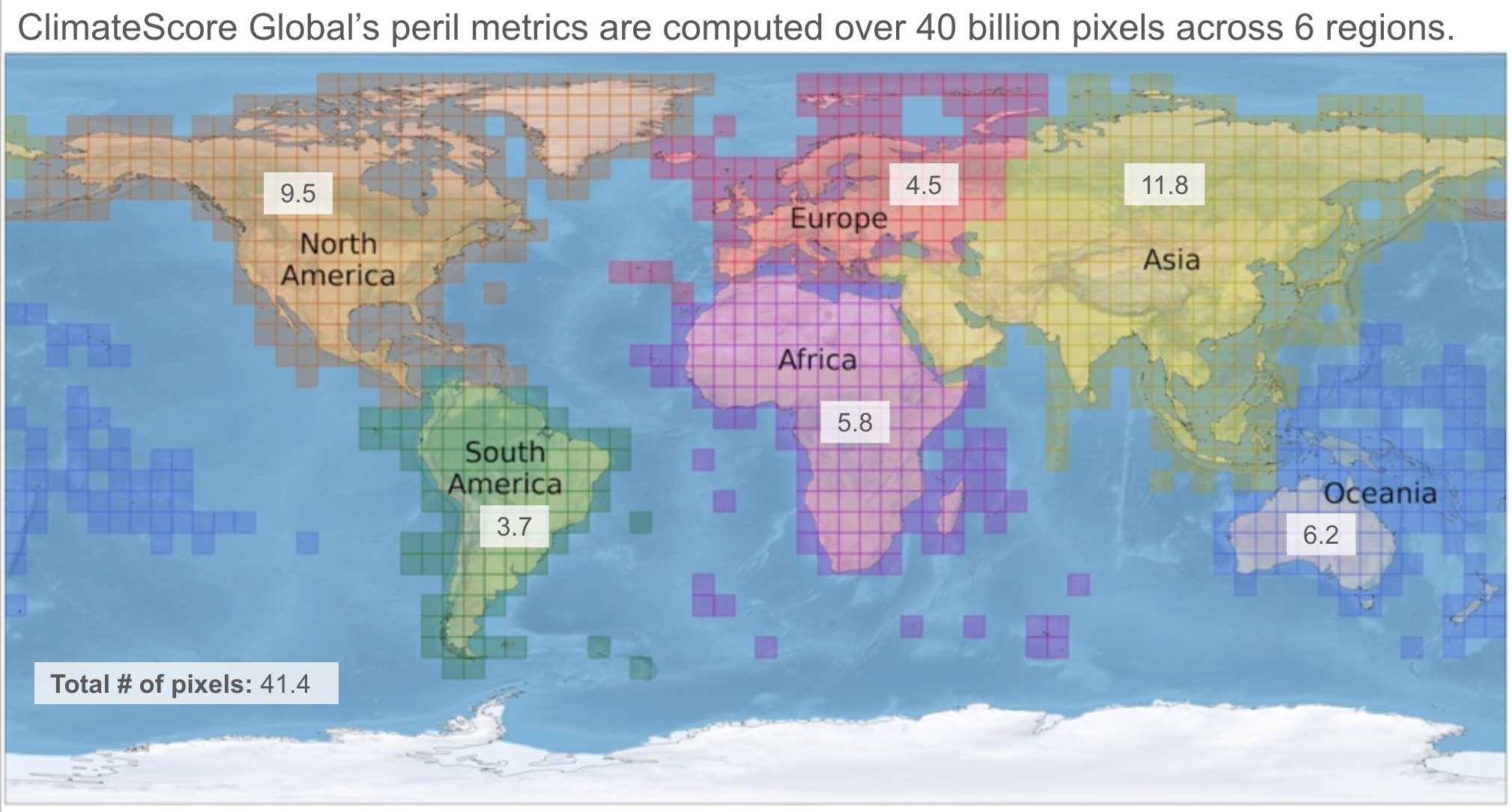
To trust climate scores or other climate analytics, a sophisticated user must feel confident that the raw physical hazards – extreme heat, wind, fire, flood – are verified, validated, and trustworthy. Jupiter’s verification and validation framework provides a regular, transparent, and rigorous methodology for testing all data produced at Jupiter. Verification and validation happens at every stage of the production pipeline for our downscaled climate model data. This way, errors are caught early and quality is ensured throughout the data production process. Jupiter’s verification and validation includes both automated processes and manual checks carried out by scientific experts. Jupiter performs dozens of individual checks against all 251 trillion data values globally. This transparent, comprehensive, quantifiable, and well-documented verification and validation process has enabled Jupiter’s climate model data to pass Model Risk Management (MRM) model validation at Tier 1 banks, allowing for the rapid adoption of decision-ready climate risk analytics. 

Verification and the Jupiter Quality Score

Verification can be thought of as the quality control process within the peril production software pipeline. While the process can be largely automated, expert judgement is required in the design of the process. Each of Jupiter’s nine climate peril models – flood, wildfire, wind, precipitation, heat, cold, drought, subsidence, and hail (severe thunderstorms) – has its own verification pipeline, with each model’s outputs closely validated by a lead scientist. Jupiter creates a list of Quality Indicators for each peril and uses them to create a final Jupiter Quality Score (JQS) for each peril. 

Creating the Jupiter Quality Score

The quality indicators for each peril include a set of general technical checks, as well as cross-level checks. These checks include quantitative data quality control, such as automatically flagging potentially invalid or non-physical data values; and expert-led qualitative review and evaluation of outputs and comparison of results to established scientific literature. General technical checks include tests such as:    

• Value consistency: Making sure that mean, minimum, and maximum data values make physical sense, based on the peril being verified;
• Uncertainty range: Ensuring the uncertainty range (5th percentile to 95th percentile) makes sense physically; that the lower bound (5th percentile) is greater than the upper bound (95th percentile); and that uncertainty is not zero;
• Flat line test: Making sure that projected values are NOT identical across future years, as this could indicate data processing errors;
• Missing data: These checks make sure that locations that should have data do have data; and that all uncertainty levels have data. 

Cross-level checks occur across different return periods, and time epochs. Like the general technical checks, the cross-level checks fuse automated detection with scientific expertise to perform both qualitative and quantitative assessments on data quality. Cross-level checks include:  

• Metric differences: This check ensures that metric values for higher return periods are higher – that is, flood depths for a 500-year flood should be greater than flood depths for a 200-year flood;
• Year difference: This check looks at metric trend values across 5-year periods, and makes sure they are reasonable based on scientific experts’ understanding of climate impacts on that specific peril;  
• Maximum trend deviations: This check looks at how much metrics change over time – unusually large changes over time could be indicative of data quality issues or non-physical artifacts introduced by downscaling. For perils that are fairly spatially continuous, such as heat and wind, spatial deviations are also analyzed, as large spatial variations could indicate a data quality problem.   
• Consistency: Finally, metrics are checked to make sure that they exist for all forecast years, and all return periods.

All these checks, when aggregated for each metric, scenario, year, uncertainty level, and location, are aggregated across epochs to produce a Jupiter Quality Score, or JQS. This quality score is a unitless verification and validation index that ranges from -100 to +100. -100 indicates a very poor score, while +100 indicates an excellent score. Scores of -101 indicate that a test cannot be performed for some reason, while a score of -200 indicates that a peril fails a fundamental data consistency test. A score between 50 and 100 is very good.

The Jupiter Quality Score in Action

To see the Jupiter Quality Score in action, we analyze the Jupiter Quality Scores (JQS) for the heat peril. The heat peril is delivered by peril metrics that estimate the ways heat can stress or threaten people, systems, and entities: human productivity and health impacts, infrastructure damage, cooling costs, and reduced operating efficiency of equipment. Heat peril metrics include acute peril metrics that estimate the impacts of extreme heat, and chronic peril metrics that estimate the impact of sustained temperature increases. 

For each Jupiter heat model metric, Jupiter experts determine subjective thresholds for the verification and validation process. For example, consider the metric daysExceeding35C, which measures the number of days per year where temperature is above 35°C. Since the metric estimates days per year that satisfy the temperature threshold, the minimum value of this metric cannot be below zero days, and the maximum value of this metric cannot be greater than 365 days. Locations where this metric is less than zero or greater than 365 will have a decrease in their JQS.

Consider a cross-level check for this same Jupiter heat metric, minimum and maximum year differences. These checks specify how much our heat metric, daysExceeding35C, can vary between 5-year periods. The minimum is set at -5, and the maximum is set at 50. This means that if daysExceeding35C decreases by more than 5 days across a 5-year period (or increases by more than 50), the JQS will be decreased.  

JQS is 100 if every check is passed at every location for every metric, scenario, year, uncertainty level, and epoch. Every time some combination of metric, scenario, year, uncertainty level, and epoch does not pass, the JQS decreases slightly. The two most common reasons for JQS to decrease are year differences, when a metric changes more or less than expected from one 5-year period to another; and maximum trend deviations, when metric changes deviate more than expected over time. 

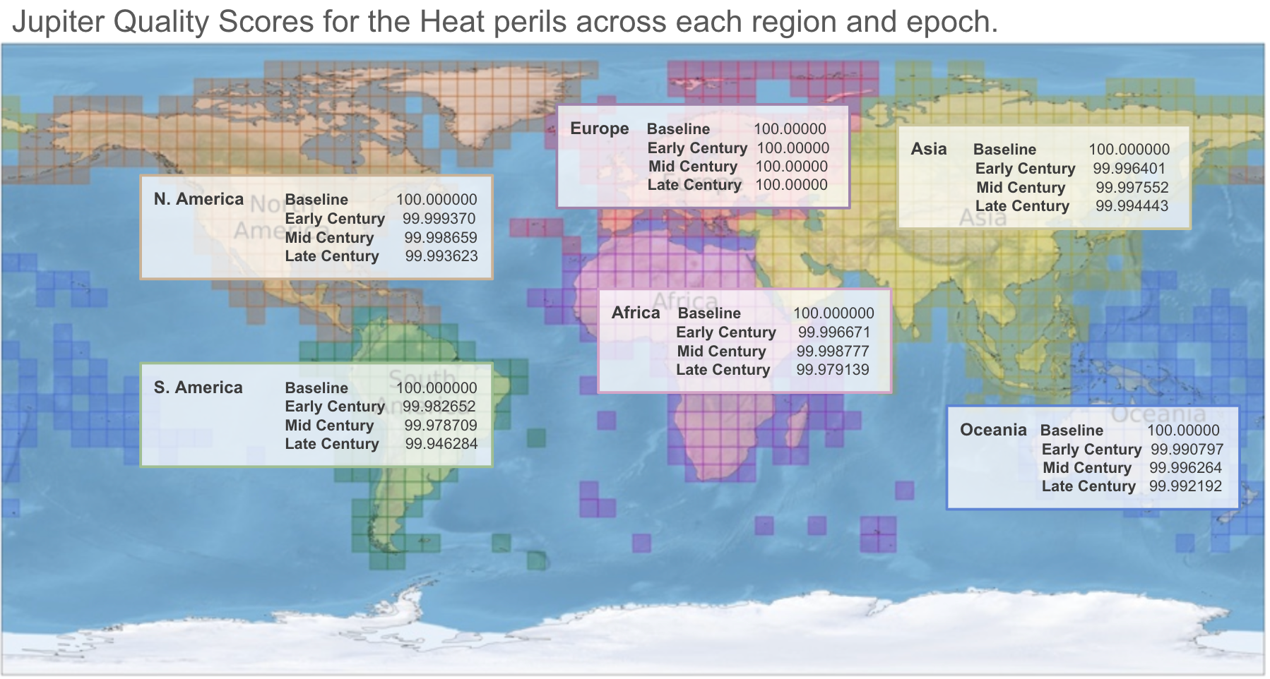
Figure 5 shows the JQS estimates for Jupiter's heat model for each region and epoch. Note that the scores in Europe are the highest. This is likely because Europe is a focal point for a lot of extreme heat research, and thus the subjective JQS thresholds may be derived from Europe-specific data. Nevertheless, the JQS for Heat remains quite high in all regions, with no one region’s scores below a 99.94. 

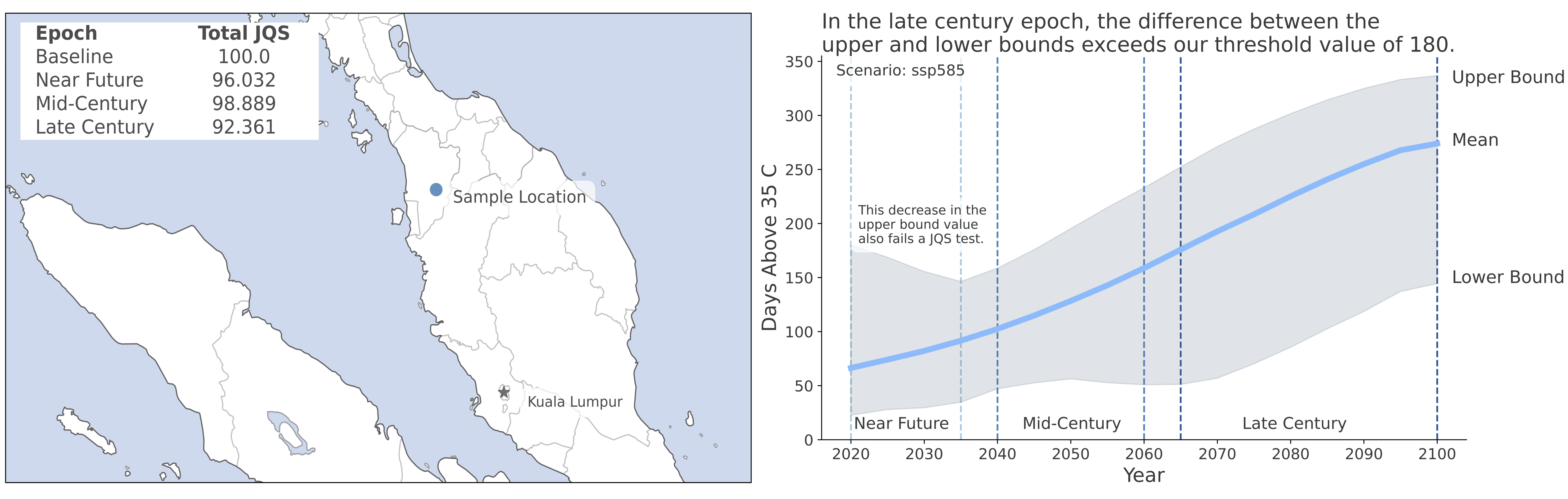
What makes a score drop below 100? To answer this question, we break down a score for a single peril (daysExceeding35C) at a single location. In this case, a location north of Kuala Lumpur in peninsular Malaysia (Figure 6). We can see in Figure 6 that our JQS for all three future epochs has dropped below 100. Let’s find out why. 

We perform our checks for the mean values as well as the upper (95th percentile) and lower (5th percentile) levels for our peril metric, daysExceeding35C. We start with our general technical checks:

1. Value consistency. Since our metric is in the units of days per year, all values must be between zero and 365. This test is passed for all scenarios and years.  
2. Uncertainty range. For this peril metric, the difference between our upper and lower bounds cannot exceed 180 days. In Figure 6, we can see that this range exceeds 180 for some of our mid-century and most of our late century epoch. This will lower our JQS for the mid- and late century epochs.  
3. Flat line.  We ensure that our peril metrics are not the exact same value every year. This test is passed for all scenarios and years.  

We passed tests 1 and 3; but test 2 failed during the mid-century and late century epochs. Next, we also look at our cross-level checks: 

4. Metric difference check. Here, we want to make sure that our metrics make sense relative to each other. For example, we estimate daysExceeding38C, in addition to daysExceeding35C. daysExceeding35C should never be less than daysExceeding38C. This test is passed for all scenarios and years.
5. Year difference. This test ensures that the metric’s change over time is reasonable, and that changes are not too big from year to year. For this peril, year-over-year changes must be between -5 and 50. In Figure 6, we can see that the upper bound on daysExceeding35C changes by more than our -5 day threshold in the near future epoch. This will lower our JQS for our near future epoch. 
6. Year difference anomaly. This test ensures that our year differences are not too different from each other, which could indicate large spikes or discontinuities in our projections. This test is passed for all scenarios and years.

Thus, we can see that two tests were failed: the uncertainty range test during the mid-century and late century epochs, and the year difference test during the near-future epochs. Ultimately, while these tests were failed, the total JQS is still high for each epoch, and the metric values are still reasonable compared to other climate projections (e.g., other downscaled CMIP6 projections).   

Validation and the Jupiter Observation Score

At Jupiter, verification refers to quality control and internal consistency checks for our high-resolution downscaled climate model data. After verification, Jupiter data undergoes a validation process. Here, validation is defined as “determining the extent to which a model represents the real world from the perspective of its intended uses” ⁹. 

Just like verification, validation is peril-specific and performed for each peril at each location under each epoch. The external datasets used for validation vary by peril, and are chosen based on scientific expertise, and coverage and comprehensiveness of the dataset. At Jupiter, we use over 30 different external, publicly available datasets throughout the validation process. These datasets include: 

• in-situ observational datasets for hydrological and meteorological variables; 
• satellite-derived datasets developed for tasks like flood detection, fire emissions tracking, land coverage, and lightning count; 
• global sea level rise projections; 
• dynamically downscaled regional climate data; 
• other datasets covering tropical cyclone tracks and watershed boundaries. 

A complete list of publicly available, external datasets used for validating and calibrating Jupiter's platform is provided in Table 2. 

Similar to the Jupiter Quality Score, validation scores are quantified for each location for every metric, scenario, year, uncertainty level, and epoch. These validation scores are compared to peril-relevant external datasets, to ensure that our platform estimates are in line with external, peer-reviewed estimates. 

For Jupiter's heat model, several different external datasets were used for validation. These include:

• Sub-daily, global gridded temperature data from the European Centre for Medium-Range Weather Forecasts Re-Analysis version 5 (ERA5), which is considered the superior reanalysis dataset for historical weather and climate¹⁰;
• Peer-reviewed scientific analysis of extreme heat metrics, such as extreme heat return periods¹¹, and estimates of energy use changes due to extreme heat^12,13; 
• Dynamically downscaled gridded global temperature datasets, such as CHELSA¹⁴.

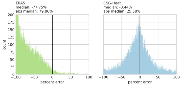
As an example, part of the validation process involves comparing our heat model to ERA5, the global standard reanalysis product, over the historical period centered on 1995. Here, we show the results for the daysExceeding35C metric, which estimates the number of days per year that exceed 35°C. We use over 30,000 in situ temperature observations across the globe (from GHCN, GSOD, AMeDAS, and CONAGUA, see Table 2) as our ground truth, and we assess both our heat model and ERA5 against this in situ weather station data. The in-situ data can better capture small scale features such as urban heat islands and topographic effects. 

When we compare our heat model and ERA5 to weather station data, we see that our dynamically downscaled heat model data more closely resembles the in-situ observations. The median percent error was -0.44%, indicating a minimal bias, while ERA5’s median percent error was -77.75%, indicating that ERA5 is consistently biased low when compared to in situ observations – a bias that has been documented in other studies^15,16. 

‍

We can also perform a spatial comparison between the Jupiter heat model and ERA5. This comparison allows us to check how the enhanced downscaling used in the model improves the representation of temperature extremes on a local scale, compared to lower-resolution datasets such as ERA5. This example, from the Chesapeake Bay in the U.S., shows that the smaller-scale topography on the land as well as the shoreline provides higher-resolution, more varied temperature estimates when compared to ERA5. 

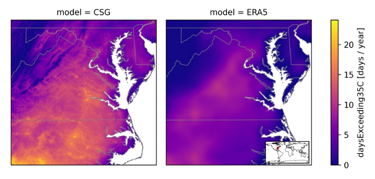
Figures 7 and 8 provide just two examples of the kinds of external data validation that our peril models undergo as part of the verification and validation process. Overall, each peril has many layers of external validation for each metric, designed and verified by peril-specific scientific experts and based on the best-available data and peer-reviewed, up-to-date scientific literature published by independent, outside scientists.  

Conclusions

For climate model data providers, generating high-resolution climate model data is only part of the process. Comprehensive, transparent, and well-documented verification and validation is a critical part of providing decision-grade climate model data. A thorough and transparent verification and validation process can provide end users and decisionmakers with confidence that their high-resolution climate model output is physically and internally consistent, is verified and analyzed by scientific experts, and compares favorably to established, peer-reviewed scientific thinking and data. 

At Jupiter, transparent, high-quality verification and validation carried out by subject matter experts is a key part of our data pipeline. In a continuing series of blog posts, we’ll discuss verification and validation in more detail for specific perils, including fire, flood, and precipitation. In these posts, we’ll discuss verification and walk through Jupiter’s external validation process in even more detail.      

References

1. IPCC, 2023: Climate Change 2023: Synthesis Report. Contribution of Working Groups I, II and III to the Sixth Assessment Report of the Intergovernmental Panel on Climate Change [Core Writing Team, H. Lee and J. Romero (eds.)]. IPCC, Geneva, Switzerland, pp. 35-115, doi:10.59327/IPCC/AR6-9789291691647. 
2. Hawkins, E., and R. Sutton, 2009: The Potential to Narrow Uncertainty in Regional Climate Predictions. Bull. Amer. Meteorol. Soc., 90, 1095 - 1108.
3. Gettleman, A., and R.B. Rood, 2016: Demystifying Climate Models–A User’s Guide to Earth System Models. Springer Nature, 274 pp. 
4. Wootten, A., A. Terando, B.J. Reich, R.P. Boyles, and F. Semazzi, 2017: Characterizing sources of uncertainty from global climate models and downscaling techniques. J. App. Meteorol. Clim., 56, 3245-3262.  
5. Otto, F., 31 October 2023: Without Warning: A Lack of Weather Stations Is Costing African Lives. Yale Environment 360. Accessed April 2, 2026. 
6. Cavazos, T., et. al., 2024: Challenges for climate change adaptation in Latin America and the Caribbean region. Front. Clim. 6:1392033. doi:10.3389/fclim.2024.1392033. 
7. Taylor, K.E., R.J. Stouffer, and G.A. Meehl, 2012: An overview of CMIP5 and the experiment design. Bull. Am. Meteorol. Soc., 93, 485–498. 
8. Eyring, V., et. al., 2016: Overview of the coupled model intercomparison project phase 6 (CMIP6) experimental design and organization. Geosci. Model Dev., 9, 1937–1958. 
9. National Research Council, Division on Engineering and Physical Sciences, Board on Mathematical Sciences and Their Applications, and Committee on Mathematical Foundations of Verification, Validation, and Uncertainty Quantification. Assessing the reliability of complex models: Mathematical and statistical foundations of verification, validation, and uncertainty quantification. National Academies Press, Washington, D.C., DC, June 2012.
10. Hersbach, H., et. al., 2020: The ERA5 global reanalysis. Q. J. R. Meteorol. Soc., 146, 1999–2049.  
11. Li., C., F. Zwiers, X. Zhang, G. Li, Y. Sun, and M. Wehner, 2021: Changes in annual extremes of daily temperature and precipitation in CMIP6 models. J. Clim., 34, 3441–3460. 
12. Petri, Y., and K. Caldeira, 2015: Impacts of global warming on residential heating and cooling degree-days in the United States. Sci. Rep., 5, 12427. 
13. Spinoni, J., et. al., 2018: Changes of heating and cooling degree-days in Europe from 1981 to 2100: HDD AND CDD IN EUROPE FROM 1981 TO 2100. Int. J. Climatol., 38, e191–e208. 
14. Karger, D.N., et. al., 2017: Climatologies at high resolution for the earth’s land surface areas. Sci. Data, 4, 170122. 
15. Lee, J., and A.E. Dessler, 2024: Improved Surface Urban Heat Impact Assessment Using GOES Satellite Data: A Comparative Study With ERA‐5. Geophys. Res. Lett., 51, e2023GL107364. 
16. Kozubek, M., P. Krizan, and J. Lastovicka, 2020: Homogeneity of the temperature data series from ERA5 and MERRA2 and temperature trends. Atmosphere (Basel), 11, 235. 

Datasets from Table 2

1. Knapp, K.R., M.C. Kruk, D.H. Levinson, H.J. Diamond, and C.J. Neumann, 2010: The international best track archive for climate stewardship (IBTrACS): Unifying tropical cyclone data. Bull. Am. Meteorol. Soc., 91, 363–376. 
2. Hall, T.M., and S. Jewson, 2007: Statistical modelling of North Atlantic tropical cyclone tracks. Tellus A, 59, 486. 
3. Bloemendaal, N., I.D. Haigh, H. de Moel, S. Muis, R.J. Haarsma, and J.C.J.H. Aerts, 2020: Generation of a global synthetic tropical cyclone hazard dataset using STORM. Sci. Data, 7, 40. 
4. Muis, S., et. al., 2020: A high-resolution global dataset of extreme sea levels, tides, and storm surges, including future projections. Front. Mar. Sci., 7, 263. 
5. Kopp, R.E., et. al., 2014: Probabilistic 21st and 22nd century sea-level projections at a global network of tide-gauge sites. Earth’s Future, 2, 383–406. 
6. Sweet, W.V., et. al., 2017: Global and Regional Sea Level Rise Scenarios for the United States. NOAA Technical Report NOS CO-OPS 083, National Oceanic and Atmospheric Administration, Silver Spring, Maryland, 55 p. 
7. Lehner, B., and G. Grill, 2013: Global river hydrography and network routing: baseline data and new approaches to study the world’s large river systems. Hydrol. Process., 27, 2171–2186. 
8. Buchhorn, M., et al. Copernicus Global Land Service: Land Cover 100m: Collection 2: Epoch 2015: Globe. V2.0.2, Zenodo, 1 Oct. 2019, doi:10.5281/zenodo.3243509. 
9. Giglio, L., J.T. Randerson, and G.R. van der Werf, 2013: Analysis of daily, monthly, and annual burned area using the fourth-generation global fire emissions database (GFED4): ANALYSIS OF BURNED AREA. J. Geophys. Res. Biogeosci., 118, 317–328. 
10. Prigent, C., C. Jimenez, and P. Bousquet, 2020: Satellite-derived global surface water extent and dynamics over the last 25 years (GIEMS-2). J. Geophys. Res., 125. 
11. Li, S., et. al., 2018: Automatic near real-time flood detection using Suomi-NPP/VIIRS data. Remote Sens. Environ., 204, 672–689. 
12. Freiler, K., et. al., 2017: Assessing the impacts of 1.5°C global warming – simulation protocol of the inter-sectoral impact model intercomparison project (ISIMIP2b). Geosci. Model Dev.,10, 4321–4345. 
13. Hanasaki, N., S. Yoshikawa, Y. Pokhrel, and S. Kanae, 2018: A global hydrological simulation to specify the sources of water used by humans. Hydrol. Earth Syst. Sci., 22, 789–817. 
14. Falcone, J.A., 2011: GAGES-II: Geospatial Attributes of Gages for Evaluating Streamflow, Dataset, https://doi.org/10.3133/70046617. 
15. Woodworth, P.L., J.R. Hunter, M. Marcos, P. Caldwell, M. Menéndez, and I. Haigh, 2016: Towards a global higher-frequency sea level dataset. Geosci. Data J., 3, 50–59. 
16. Center for Operational Oceanographic Products and Services (CO-OPS). NOAA Water Levels Dataset, [https://tidesandcurrents.noaa.gov/stations.html?type=Water+Levels].
17. Caldwell, P. C., M. A. Merrifield, P. R. Thompson, 2015: Sea level measured by tide gauges from global oceans — the Joint Archive for Sea Level holdings (NCEI Accession 0019568), Version 5.5, NOAA National Centers for Environmental Information, Dataset, doi:10.7289/V5V40S7W. 
18. Japan Meteorological Agency. Automated Meteorological Data Acquisition System (AMeDAS). Dataset, https://www.data.jma.go.jp/obd/stats/etrn/index.php. 
19. Menne, M.J., et. al., 2012: Global historical climatology network - daily (GHCN-daily), version 3. [link]
20. Smith, A., N. Lott, and R. Vose, 2011: The integrated surface database: Recent developments and partnerships. Bull. Am. Meteorol. Soc., 92(6):704–708. 
21. Comisión Nacional del Agua (CONAGUA). Geoportal Sistema Nacional de Información del Agua. 
22. Météo-France. Données climatologiques de base. Dataset,  https://meteo.data.gouv.fr/datasets?category=climatologique-base 
23. Huerta, A., R. Serrano-Notivoli, and S. Brönnimann, 2025: SC-PREC4SA: A serially complete daily precipitation dataset for South America. Sci. Data, 12(1):1006. 
24. Perica, S., et al. "Precipitation-Frequency Atlas of the United States, Volume 11 Version 2.0: Texas", 2018, https://doi.org/10.25923/1ceg-5094. 
25. Bonnin, G.M., et al. "Precipitation-Frequency Atlas of the United States, Volume 1 Version 5.0: Semiarid Southwest (Arizona, Southeast California, Nevada, New Mexico, Utah)", 2004. https://repository.library.noaa.gov/view/noaa/22609. 
26. Bonnin, G.M., et al. "Precipitation-Frequency Atlas of the United States, Volume 2 Version 3.0: Delaware, District of Columbia, Illinois, Indiana, Kentucky, Maryland, New Jersey, North Carolina, Ohio, Pennsylvania, South Carolina, Tennessee, Virginia, West Virginia", 2004. https://repository.library.noaa.gov/view/noaa/22610.  
27. Perica, S., et al. "Precipitation-Frequency Atlas of the United States, Volume 6 Version 2.3: California", 2011. https://repository.library.noaa.gov/view/noaa/22614. 
28. Perica, S., et al. "Precipitation-Frequency Atlas of the United States, Volume 8 Version 2.0: Midwestern States (Colorado, Iowa, Kansas, Michigan, Minnesota, Missouri, Nebraska, North Dakota, Oklahoma, South Dakota, Wisconsin)" , 2013. https://repository.library.noaa.gov/view/noaa/22616. 
29. Perica, S., et al. "Precipitation-Frequency Atlas of the United States, Volume 9 Version 2.0: Southeastern States, Alabama, Arkansas, Florida, Georgia, Louisiana, Mississippi" , 2013. https://repository.library.noaa.gov/view/noaa/22617 
30. Perica, S., et al. "Precipitation-Frequency Atlas of the United States. Volume 10, Version 3.0. Northern States; Connecticut, Maine, Massachusetts, New Hampshire, New York, Rhode Island, Vermont", 2015, https://doi.org/10.25923/99jt-a543. 
31. Stratton, R.A., et al., 2018: "A Pan-African convection-permitting regional climate simulation with the Met Office Unified Model: CP4-Africa." J. Climate, 31, 3485-3508. 
32. Leutwyler, D., et al., 2017: Evaluation of the convection‐resolving climate modeling approach on continental scales. J. Geophys. Res.: Atmos., 122, 5237-5258. 
33. Liu, C., et al., 2017: Continental-scale convection-permitting modeling of the current and future climate of North America. Climate Dynamics 49, 71-95. 
34. Sasai, T., et al., 2019: Future projection of extreme heavy snowfall events with a 5‐km large ensemble regional climate simulation. J. Geophys. Res.: Atmos., 124, 13975-13990. 
35. Cecil, D.J., D.E. Buechler, and R.J. Blakeslee, 2014: Gridded lightning climatology from TRMM-LIS and OTD: Dataset description. Atmos. Res., 135, 404–414. 
36. Peterson, M., D. Mach, and D. Buechler, 2021: A global LIS/OTD climatology of lightning flash extent density. J. Geophys. Res., 126, e2020JD033885. 
37. Boussetta, S., G. Balsamo, A. Beljaars, T. Kral, and L. Jarlan, 2013: Impact of a satellite-derived leaf area index monthly climatology in a global numerical weather prediction model. Int. J. Remote Sens., 34, 3520–3542. 

‍